Returns of financial stocks
This project, realized in collaboration with my study group at London Business Schoo, explores the returns of some stocks, we will also have the opportunity to construct our own portfolio and plot it.
As usual, we will look first at our dataset to understand it better and ensure there is no missing or duplicated values.
#Loading the data and getting its Summary
nyse <- read_csv(here::here("data","nyse.csv"))

skim(nyse)| Name | nyse |
| Number of rows | 508 |
| Number of columns | 6 |
| _______________________ | |
| Column type frequency: | |
| character | 6 |
| ________________________ | |
| Group variables | None |
Variable type: character
| skim_variable | n_missing | complete_rate | min | max | empty | n_unique | whitespace |
|---|---|---|---|---|---|---|---|
| symbol | 0 | 1 | 1 | 4 | 0 | 508 | 0 |
| name | 0 | 1 | 5 | 48 | 0 | 505 | 0 |
| ipo_year | 0 | 1 | 3 | 4 | 0 | 33 | 0 |
| sector | 0 | 1 | 6 | 21 | 0 | 12 | 0 |
| industry | 0 | 1 | 5 | 62 | 0 | 103 | 0 |
| summary_quote | 0 | 1 | 31 | 34 | 0 | 508 | 0 |
Fortunately, we can keep the data as is.
To start our analysis, we will rank the number of stocks in each sector.
# Grouping the companies by sector, counting the number of companies in each sector and arranging the data in descending order
stocks <- data.frame(nyse) %>%
  group_by(sector) %>%
  count(sort=TRUE)

# Plotting the number of companies listed in the NYSE by sector

ggplot(data = stocks, aes(y= reorder(sector,n), x=n))+
  geom_bar(stat='identity')+
  labs(
    x="Number of companies",
    y="Sector",
    title = "Number of companies listed in the NYSE by sector")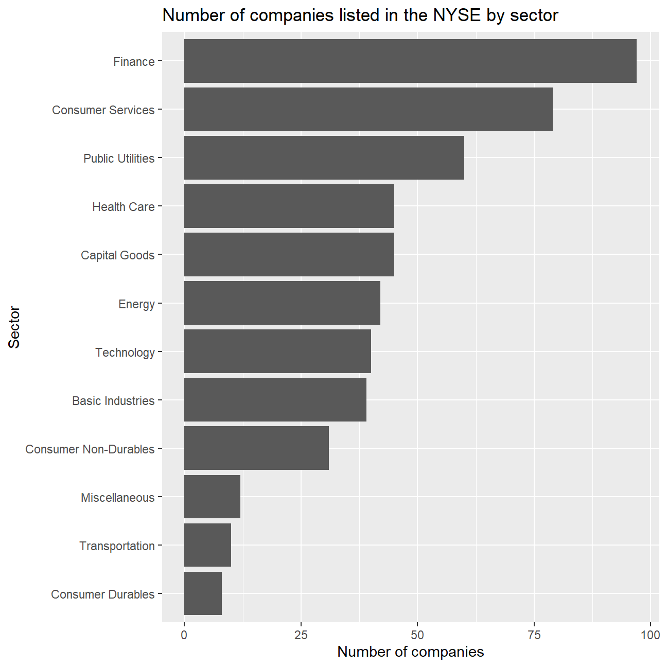
To continue our analysis, we are choosing six stocks “BLK”, “JPM”, “CS”, “GS”, “MS”, “RY”, “UBS”, “SPY”.
# Notice the cache=TRUE argument in the chunk options. Because getting data is time consuming,
# cache=TRUE means that once it downloads data, the chunk will not run again next time you knit your Rmd

#Adding our stocks in myStocks to later use this group for the analysis

myStocks <- c("BLK","JPM","CS","GS","MS","RY","UBS","SPY" ) %>%
  tq_get(get  = "stock.prices",
         from = "2011-01-01",
         to   = "2020-08-31") %>%
  group_by(symbol)

glimpse(myStocks) # examine the structure of the resulting data frame
## Rows: 18,463
## Columns: 8
## Groups: symbol [8]
## $ symbol <chr> "BLK", "BLK", "BLK", "BLK", "BLK", "BLK", "BLK", "BLK", "B...
## $ date <date> 2011-01-03, 2011-01-04, 2011-01-05, 2011-01-06, 2011-01-0...
## $ open <dbl> 192, 191, 190, 193, 192, 188, 192, 195, 194, 195, 199, 196...
## $ high <dbl> 195, 192, 193, 193, 192, 192, 196, 195, 196, 199, 200, 197...
## $ low <dbl> 190, 189, 189, 188, 185, 187, 191, 191, 192, 194, 194, 191...
## $ close <dbl> 190, 190, 192, 190, 188, 191, 193, 194, 196, 199, 197, 192...
## $ volume <dbl> 1085200, 794400, 925300, 727300, 886200, 898300, 734000, 8...
## $ adjusted <dbl> 145, 145, 147, 145, 144, 146, 148, 148, 149, 152, 150, 146...#calculate daily returns
myStocks_returns_daily <- myStocks %>%
tq_transmute(select = adjusted,
mutate_fun = periodReturn,
period = "daily",
type = "log",
col_rename = "daily_returns",
cols = c(nested.col))
#calculate monthly returns
myStocks_returns_monthly <- myStocks %>%
tq_transmute(select = adjusted,
mutate_fun = periodReturn,
period = "monthly",
type = "arithmetic",
col_rename = "monthly_returns",
cols = c(nested.col))
#calculate yearly returns
myStocks_returns_annual <- myStocks %>%
group_by(symbol) %>%
tq_transmute(select = adjusted,
mutate_fun = periodReturn,
period = "yearly",
type = "arithmetic",
col_rename = "yearly_returns",
cols = c(nested.col))Now we want to see the performance of our chosen stocks.
#Summarising the information about the monthly returns of the chosen stocks and calculating the min,max, median, mean and SD for each of the companies
  analysis<- myStocks_returns_monthly %>%
  summarize(
    mean_return=mean(monthly_returns),
    median_return=median(monthly_returns),
    sd_return=sd(monthly_returns),
    min_return=min(monthly_returns),
    max_return=max(monthly_returns))%>%
  arrange(desc(mean_return))
For our last two analysis, we will first plot the density of monthly returns for each stock.
# Plotting a density chart of the monthly returns for each of the stocks
ggplot(myStocks_returns_monthly,
       aes(x= monthly_returns*100))+
  geom_density(kernel="gaussian")+
  labs(
    title="Density of Monthly Returns",
    x="Monthly Return(in %)",
    y="Density") +
  facet_wrap(~symbol)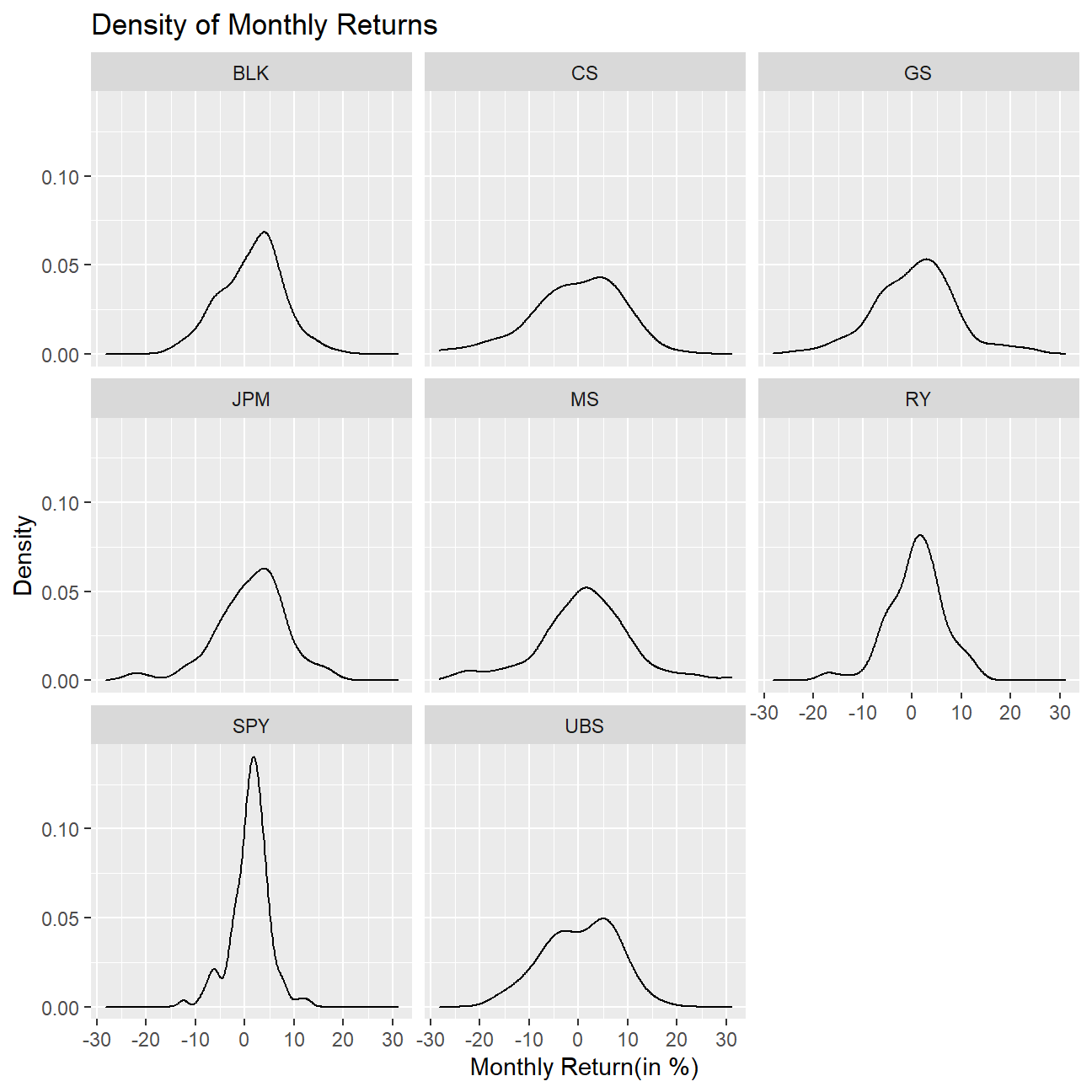
What can you infer from this plot? Which stock is the riskiest? The least risky?
From the plot it is clear to see that the individuals stocks are more risky than the ETF as their returns are more variable. Morgan Stanley is the riskiest stock with a volatility (standard deviation of the monthly returns) of 9.28% and the least risky, as it was expected, is the SPY Index with a volatility of 3.81%. This was expected since the ETF is a combination of 500 stocks, which has its systematic risk lowered through diversification.
Lastly, we have a look at the standard deviation against the mean for our six stocks.
#Plotting the standard deviation against the mean return for the stocks chosen
ggplot(analysis,
       aes(
         x=sd_return*100,
         y=mean_return*100,
         label= symbol))+
  geom_point() +
  geom_text_repel()+
  labs(
    title="Relation between the Mean Return and Standard Deviation",
    x="Standard Deviation (in %)",
    y="Mean Return (in %)")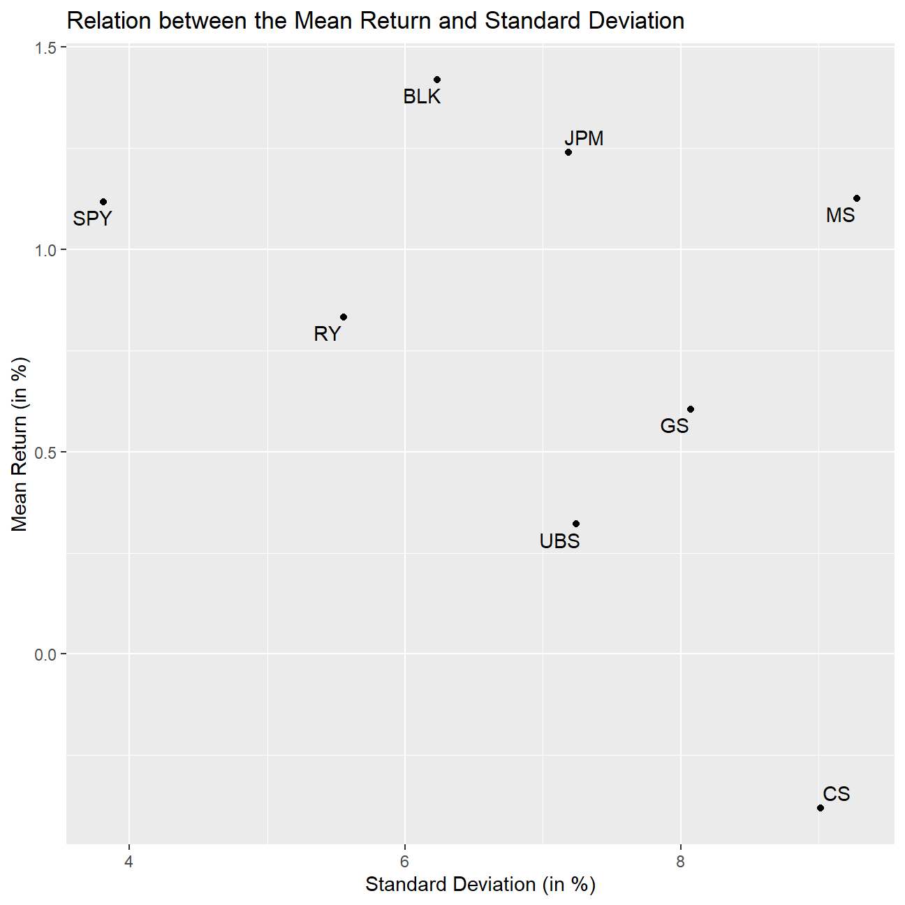
From the plot we can see that CS is the worst performing stock within this group and it is the second most risky, which means that it has the lowest sharpe ratio (Return/Volatility), this way, it would have been the worst choice. On the other hand, you can also see that BlackRock (BLK) is the one with the greatest mean return while having a medium volatility compared to its peers. Lastly, comparing Morgan Stanley (MS) with SPY, it’s clear to see that it would not have been worth to invest in it as the historical mean returns of both assets were similar.