Climate Change Anomalies

Plotting Information

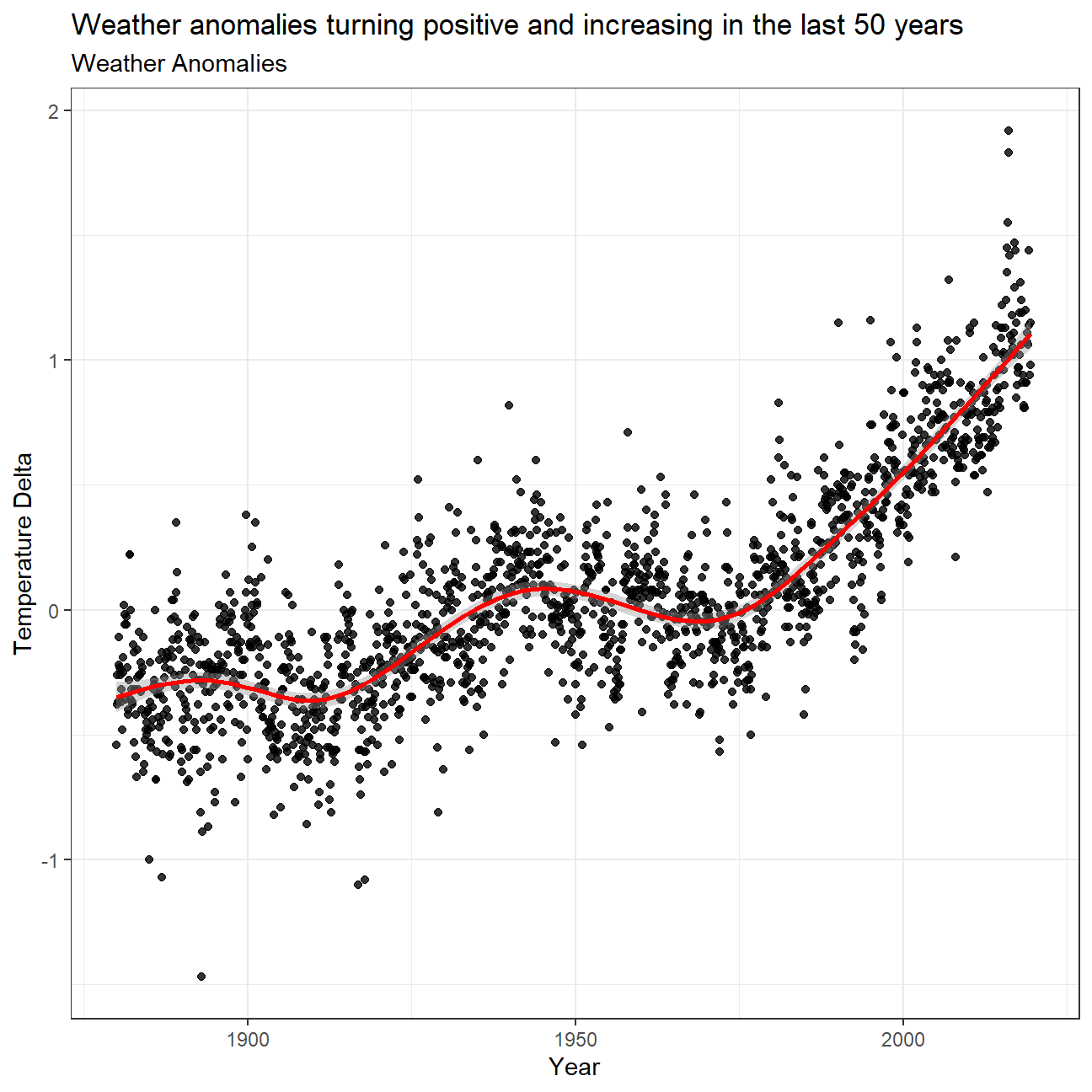
Let us plot the data using a time-series scatter plot, and add a trendline. To do that, we first need to create a new variable called date in order to ensure that the delta values are plot chronologically.

# Filtering the dates
tidyweather <- tidyweather %>%
  mutate(date = ymd(paste(as.character(Year), month, "1")),
         month = month(date, label=TRUE),
         year = year(date))

# Constructing the grpah 
ggplot(tidyweather, aes(x=date, y = delta))+
  geom_point(alpha=0.8)+
  geom_smooth(color="red") +
  theme_bw() +
  labs (title = "Weather anomalies turning positive and increasing in the last 50 years",
    subtitle = "Weather Anomalies", 
    x = "Year", 
    y= "Temperature Delta"
  )

This trend could be different depending on the month. Thus we’ll have a look at the same kind of graph but this time faceted by month.

ggplot(tidyweather, aes(x=date, y = delta))+
  geom_point()+
  geom_smooth(color="red") +
  theme_bw() +
  labs (title = "Weather anomalies changes are constant throughout the months",
    subtitle = "Weather Anomalies", 
    x="Year", 
    y="Temperature Delta"
  )+
  facet_wrap(~month)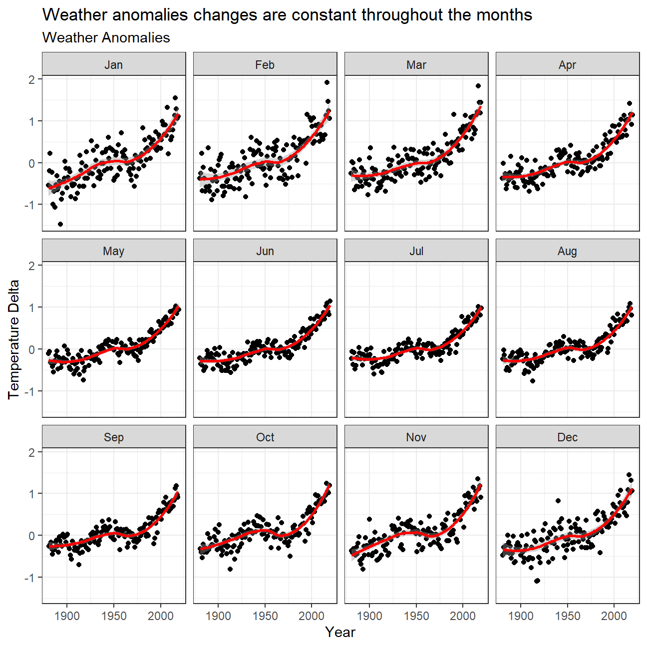

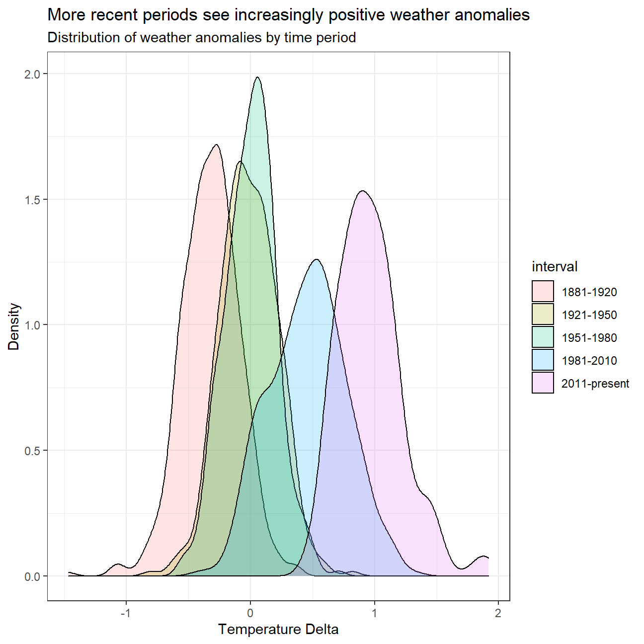
It is sometimes useful to group data into different time periods to study historical data. For example, we often refer to decades such as 1970s, 1980s, 1990s etc. to refer to a period of time. NASA calculates a temperature anomaly, as difference form the base period of 1951-1980. The code below creates a new data frame called comparison that groups data in five time periods: 1881-1920, 1921-1950, 1951-1980, 1981-2010 and 2011-present.

We remove data before 1800 and before using filter. Then, we use the mutate function to create a new variable interval which contains information on which period each observation belongs to. We can assign the different periods using case_when().

comparison <- tidyweather %>% 
  filter(Year>= 1881) %>%     #remove years prior to 1881
  #create new variable 'interval', and assign values based on criteria below:
  mutate(interval = case_when(
    Year %in% c(1881:1920) ~ "1881-1920",
    Year %in% c(1921:1950) ~ "1921-1950",
    Year %in% c(1951:1980) ~ "1951-1980",
    Year %in% c(1981:2010) ~ "1981-2010",
    TRUE ~ "2011-present"
  ))

Now that we have the interval variable, we can create a density plot to study the distribution of monthly deviations (delta), grouped by the different time periods we are interested in.

ggplot(comparison, aes(x=delta, fill=interval))+
  geom_density(alpha=0.2) +   #density plot with tranparency set to 20%
  theme_bw() +                #theme
  labs (
    title = "More recent periods see increasingly positive weather anomalies",
     subtitle = "Distribution of weather anomalies by time period",
    y = "Density"         #changing y-axis label to sentence case
    ,x = "Temperature Delta"
  )

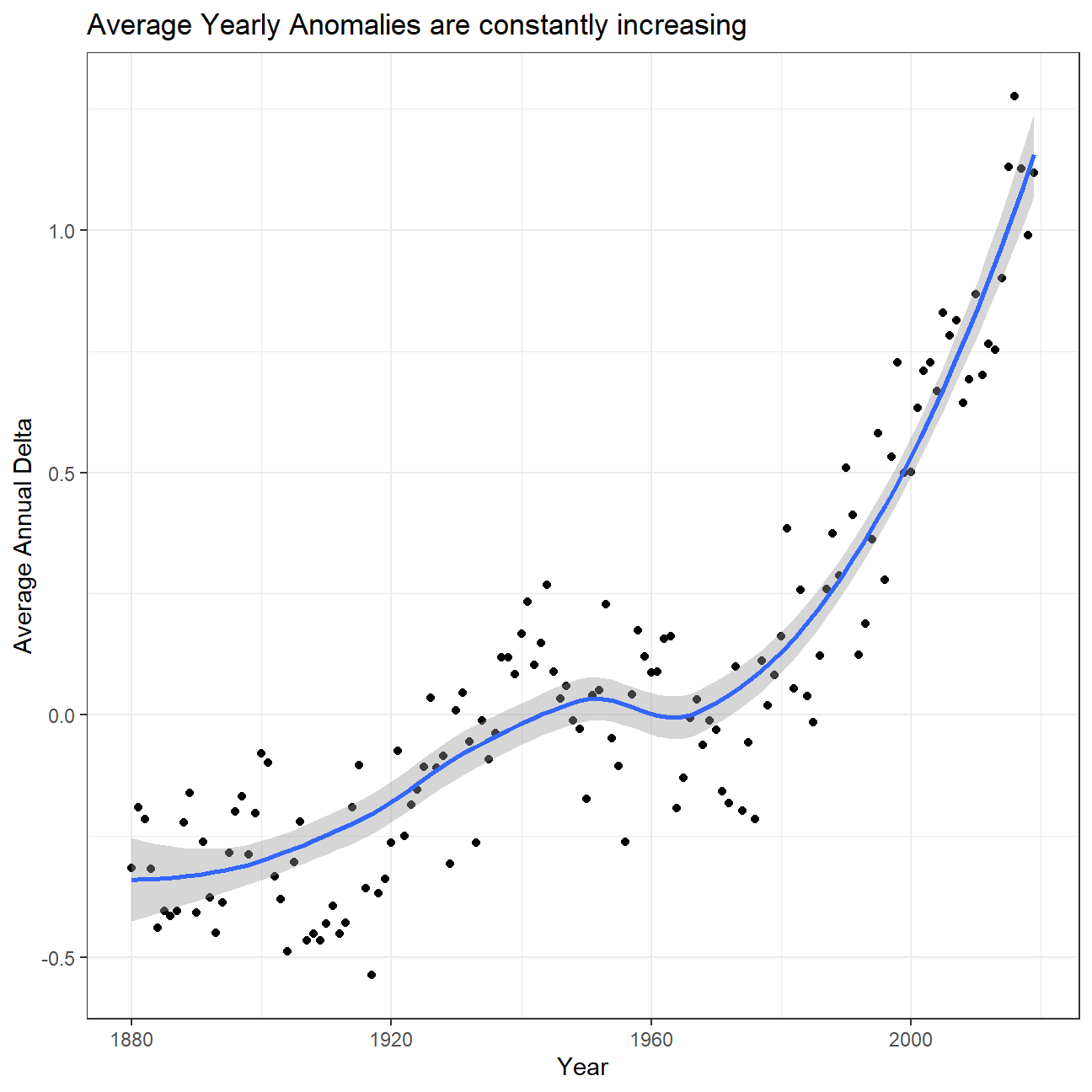
So far, we have been working with monthly anomalies. However, we might be interested in average annual anomalies. We can do this by using group_by() and summarise(), followed by a scatter plot to display the result.

#creating yearly averages
average_annual_anomaly <- tidyweather %>% 
  group_by(Year) %>%   #grouping data by Year
  
  # creating summaries for mean delta 
  # use `na.rm=TRUE` to eliminate NA (not available) values 
  summarise(annual_average_delta = mean(delta, na.rm=TRUE)) 

#plotting the data:
ggplot(average_annual_anomaly, aes(x=Year, y= annual_average_delta))+
  geom_point()+
  
  #Fit the best fit line, using LOESS method
  geom_smooth() +
  
  #change to theme_bw() to have white background + black frame around plot
  theme_bw() +
  labs (
    title = "Average Yearly Anomalies are constantly increasing",
    y     = "Average Annual Delta"
  )                         

Confidence Interval for delta

We are now going to construct a confidence interval for the average annual delta since 2011, both using a formula and using a bootstrap simulation with the infer package.

formula_ci <- comparison %>% 

  # choose the interval 2011-present
  filter(interval == "2011-present") %>%
  filter(!is.na(delta)) %>% 
  # na.omit() %>% 
 
  # what dplyr verb will you use? 

  # calculate summary statistics for temperature deviation (delta) 
  # calculate mean, SD, count, SE, lower/upper 95% CI
  summarise(mean_delta=mean(delta),
            sd_delta=sd(delta), 
            count=n(),
            t_critical = qt(0.975, count-1),
            se_delta = sd(delta)/sqrt(count),
            margin_of_error = t_critical * se_delta,
            delta_low = mean_delta - margin_of_error,
            delta_high = mean_delta + margin_of_error)
  # what dplyr verb will you use? 

#print out formula_CI
formula_ci %>% tbl_df %>% rmarkdown::paged_table()

# use the infer package to construct a 95% CI for delta
set.seed(1234)

boot_deltas <- comparison %>% 
  filter(interval == "2011-present") %>%
  filter(!is.na(delta)) %>% 
  specify(response = delta) %>% 
  generate(reps = 1000, type = "bootstrap") %>% 
  calculate(stat = "mean")

percentile_ci <- boot_deltas %>% 
  get_confidence_interval(level = 0.95, type = "percentile") 



percentile_ci %>% tbl_df %>% rmarkdown::paged_table()

formula_ci %>% 
  select(delta_low, delta_high) %>% tbl_df %>% rmarkdown::paged_table()

The mean delta over the last 10 years is 0.966 - a significant change based on NASA’s findings. Both confidence interval methods give almost comparable results. Looking at the bootstrap method, the 95% confidence interval is between 0.917 and 1.02. This means that when looking at weather anomalies, the vast majority will over around this “one-degree” change, meaning the climate is deregulated and this will have devastating consequences.