My Future Watch List

Nowadays I don’t really have the time to watch movies. My courses at London Business School are taking most of my time and the rest of my days are dedicated to my applications to Investment Banks for a summer analyst position.

So I thought, why not already compile a list of movies to watch once the exams are behind me and my internship found.

In order to construct such a list, I am going to explore the data movies used during our first assignment in Data Analytics in Finance.

Let’s first remind ourselves the composition of the data set.

# Reading the data and analyzing the information
movies <- read_csv(here::here("data", "movies.csv"))

# I use glimpe and skim to explore the data
skim(movies)

(#tab:load_movies)Data summary

Name	movies
Number of rows	2961
Number of columns	11
_______________________
Column type frequency:
character	3
numeric	8
________________________
Group variables	None

Variable type: character

skim_variable	n_missing	complete_rate	min	max	empty	n_unique	whitespace
title	0	1	1	83	0	2907	0
genre	0	1	5	11	0	17	0
director	0	1	3	32	0	1366	0

Variable type: numeric

skim_variable	n_missing	complete_rate	mean	sd	p0	p25	p50	p75	p100	hist
year	0	1	2.00e+03	9.95e+00	1920.0	2.00e+03	2.00e+03	2.01e+03	2.02e+03	▁▁▁▂▇
duration	0	1	1.10e+02	2.22e+01	37.0	9.50e+01	1.06e+02	1.19e+02	3.30e+02	▃▇▁▁▁
gross	0	1	5.81e+07	7.25e+07	703.0	1.23e+07	3.47e+07	7.56e+07	7.61e+08	▇▁▁▁▁
budget	0	1	4.06e+07	4.37e+07	218.0	1.10e+07	2.60e+07	5.50e+07	3.00e+08	▇▂▁▁▁
cast_facebook_likes	0	1	1.24e+04	2.05e+04	0.0	2.24e+03	4.60e+03	1.69e+04	6.57e+05	▇▁▁▁▁
votes	0	1	1.09e+05	1.58e+05	5.0	1.99e+04	5.57e+04	1.33e+05	1.69e+06	▇▁▁▁▁
reviews	0	1	5.03e+02	4.94e+02	2.0	1.99e+02	3.64e+02	6.31e+02	5.31e+03	▇▁▁▁▁
rating	0	1	6.39e+00	1.05e+00	1.6	5.80e+00	6.50e+00	7.10e+00	9.30e+00	▁▁▆▇▁

glimpse(movies)

## Rows: 2,961
## Columns: 11
## $ title               <chr> "Avatar", "Titanic", "Jurassic World", "The Ave...
## $ genre               <chr> "Action", "Drama", "Action", "Action", "Action"...
## $ director            <chr> "James Cameron", "James Cameron", "Colin Trevor...
## $ year                <dbl> 2009, 1997, 2015, 2012, 2008, 1999, 1977, 2015,...
## $ duration            <dbl> 178, 194, 124, 173, 152, 136, 125, 141, 164, 93...
## $ gross               <dbl> 7.61e+08, 6.59e+08, 6.52e+08, 6.23e+08, 5.33e+0...
## $ budget              <dbl> 2.37e+08, 2.00e+08, 1.50e+08, 2.20e+08, 1.85e+0...
## $ cast_facebook_likes <dbl> 4834, 45223, 8458, 87697, 57802, 37723, 13485, ...
## $ votes               <dbl> 886204, 793059, 418214, 995415, 1676169, 534658...
## $ reviews             <dbl> 3777, 2843, 1934, 2425, 5312, 3917, 1752, 1752,...
## $ rating              <dbl> 7.9, 7.7, 7.0, 8.1, 9.0, 6.5, 8.7, 7.5, 8.5, 7....

Fortunately, there is no missing values in the data set. It is also already cleaned and tidy. However, we see that there are some duplicates so let’s remove them. I am going to remove these duplicates.

# Removing duplicates
movies_new <- movies %>% 
  distinct(title, .keep_all= TRUE)

I can now begin my analysis.

I will begin by filtering the movies by the year of production, I want to focus my attention to the most recent blockbusters since 2000. Then, I’ll see the distribution for each year and by year of the number of movies.

movies_new <- movies_new %>%
  filter(year >= 2000)

# Creating a plot
ggplot(movies_new, 
       aes(
         x = year)) +
  # Designing the graph 
  geom_histogram(fill = "cyan", colour = "black", alpha = 0.4)+
  
  # Labeling the axes
  labs(
    x = "Year", 
    y = " Count", 
    title = "Most are produce evenly among the years"
  )

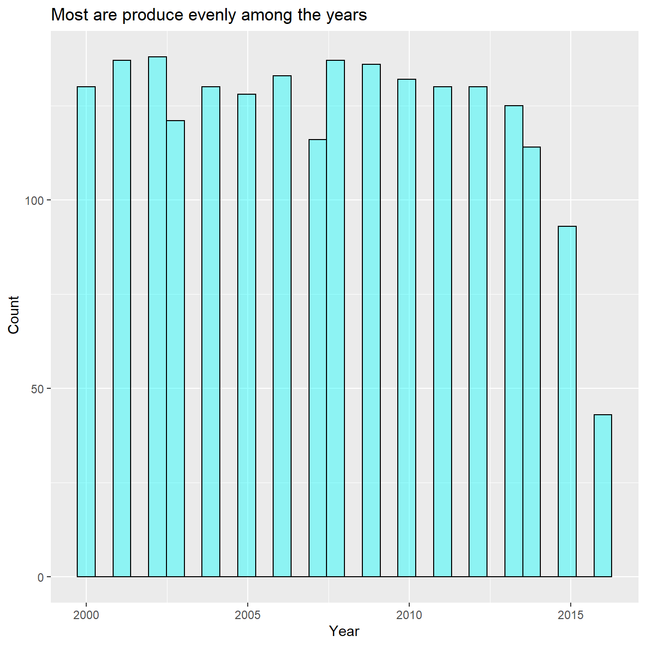We see that the movies are well spread over the years, expect for two years. I now want to see the genre categories with the most movies.

# Counting by genre
movies_new %>%
  count(genre) %>%
  # Arranging in descending order
  arrange(desc(n))

## # A tibble: 16 x 2
##    genre           n
##    <chr>       <int>
##  1 Comedy        616
##  2 Action        500
##  3 Drama         352
##  4 Adventure     206
##  5 Crime         127
##  6 Biography      98
##  7 Horror         93
##  8 Animation      27
##  9 Documentary    22
## 10 Mystery        14
## 11 Fantasy         9
## 12 Sci-Fi          4
## 13 Romance         2
## 14 Family          1
## 15 Thriller        1
## 16 Western         1

Also, I like very long movies, I’ll thus filter by duration and take movies that last only 2h30 or more.

# Filtering movies over 150 minutes in duration
movies_new <- movies_new %>% 
  filter(duration > 150)

I would like to have an idea of the rating average among the genres, I will only watch movies from the four highest ranked genre in our data set. Let’s use a boxplot to see this.

# Plotting movies by genre
ggplot(movies_new, 
       aes( 
         x = reorder(genre, rating), 
         y = rating, 
         colour = genre)) +
  geom_boxplot() +
  
  # Labeling the axes
  labs(
    title = "Adventure and Crime are the highest rated categories in our sample", 
    y = "Rating", 
    x = "Genre") +
  
  # Setting the theme and removing the legend
  theme_bw() + 
  theme(legend.position = "none")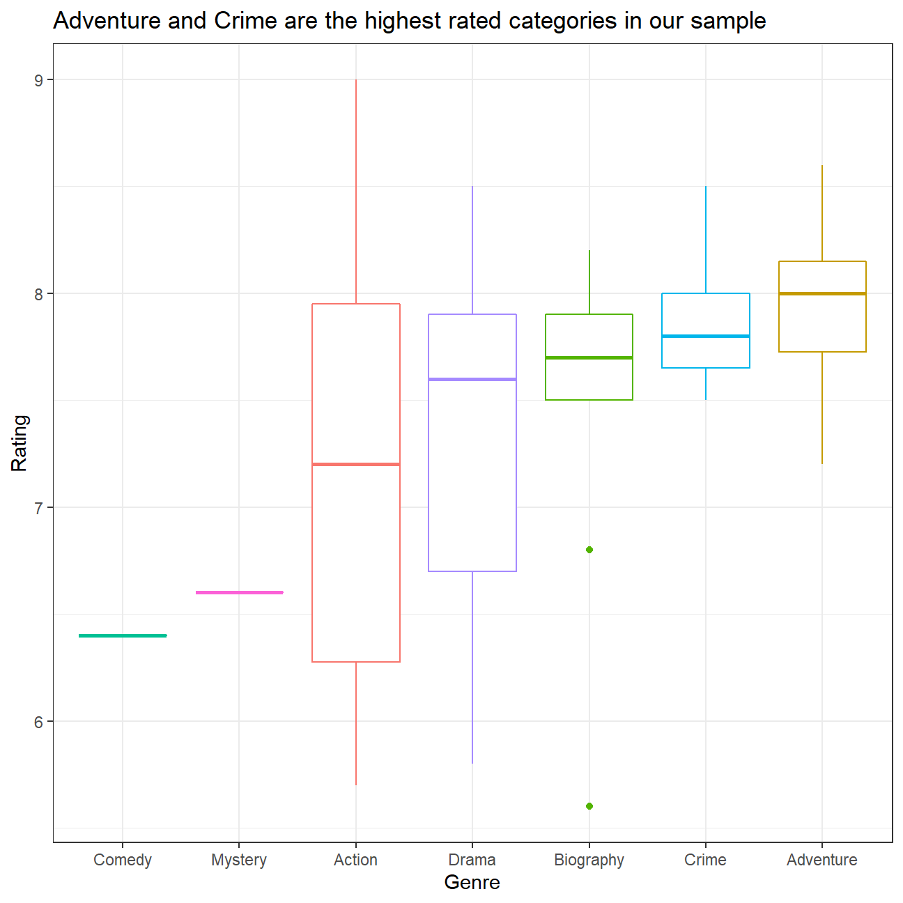

As said earlier, I am now removing the three least well rated genre.

# Remove Comedy and Mystery
movies_final <- movies_new %>% 
  filter(genre %in% c("Drama", "Biography", "Crime", "Adventure"))

However, if I keep my list as such, I will simply have too much movies on it. I need to find a way to reduce it. I think that the number of facebook likes might be of interest, and I’ll also only select movies with a rating higher than 7.5.

movies_final <- movies_final %>%
  select(title, cast_facebook_likes,  year, rating, duration, genre) %>% 
  filter(rating > 7.5) %>% 
  arrange(desc(cast_facebook_likes)) 

movies_final %>% tbl_df %>% rmarkdown::paged_table()

And voila, I now have my watch list, I’ll watch the movies in order of facebook likes.

For fun, I’ll also calculate the time needed to complete my watch list, in terms of hours but also in terms of days, assuming I can watch 8 hours per day.

movies_duration <- movies_final %>%
  group_by(genre) %>% 
  summarise(total_time = sum(duration)/60, 
            days = total_time/8) %>% 
  arrange(desc(total_time))

movies_duration %>% tbl_df %>% rmarkdown::paged_table()

We see that I will watch mostly Crime movies in terms of duration, with no less than 2 days to complete this single genre.

I cannot wait to begin the first movie: The Revenant with Leonardo Di Caprio.